4.3. Benchmarking
This section contains a series of examples performed in a Linux box with a 1.7 GHz Dual core processor. At least 256 Mb RAM are required to repeat some of these examples.
We use the external executable xperm, compiled from the code xperm.c and linked from xPerm` through the MathLink protocol (xperm.tm template). The code xperm.c contains some C99 extensions, supported by GNU gcc, and therefore Linux and Mac can always use this executable. However, all other Windows C-compilers that MathLink can communicate to (Borland, MS Visual 2003, etc) are still C90 complier only. The gcc compiler under Windows (under the cygwin system) is compatible with MathLink only from version 6.0 of Mathematica, but not before and therefore pre-6.0 versions of Mathematica cannot use xperm.
This variable says whether the connection to the external executable has been performed correctly. If you get False, don't try to repeat these examples; they will take too long.
In[259]:=
![]()
Out[259]=
![]()
Example 1:
Let us come back to the problem of products of antisymmetric tensors.
This simple code constructs the products we want to canonicalize:
In[260]:=
![]()
In[261]:=
![]()
Out[261]=
![]()
In[262]:=
![]()
Out[262]=
![]()
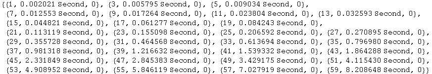
We shall need up to 59 different indices:
In[263]:=
![]()
Out[263]=

And this canonicalizes it, giving the AbsoluteTiming spent. Note that we can get products of up to 25 tensors in less than half a second (in that case the dummy group D has more than 5 10^32 elements).
In[264]:=
![]()
In[265]:=
![]()
Out[265]=
![]()
In[266]:=
![]()
Out[266]=
![]()
In[267]:=
![]()
Out[267]=
![]()
Let us see how the timings scale with the number of antisymmetric tensors. Evaluating this cell takes about a minute in a 1.8GHz Dual core processor. The executable xperm.linux requires here up to 30 Mbytes. Each computation is done only once, and that invariably introduces small deviations depending on which other tasks the computer is busy with.
In[268]:=
![]()
Out[268]=
In[269]:=
![]()
Out[269]//TableForm=
| n | time | result |
| 1 | 0.00202.757111307011273 Second | 0 |
| 3 | 0.005795.214598433795589 Second | 0 |
| 5 | 0.009034.407425079721348 Second | 0 |
| 7 | 0.01255.550292522320793 Second | 0 |
| 9 | 0.01726.688686420834812 Second | 0 |
| 11 | 0.02380.828194935088728 Second | 0 |
| 13 | 0.03259.964669330134251 Second | 0 |
| 15 | 0.044821.103026535334396 Second | 0 |
| 17 | 0.061277.238842488447243 Second | 0 |
| 19 | 0.084243.377078817725707 Second | 0 |
| 21 | 0.11312.5050805506948945 Second | 0 |
| 23 | 0.15510.642151191086727 Second | 0 |
| 25 | 0.20659.766658493529896 Second | 0 |
| 27 | 0.27089.8843459826839934 Second | 0 |
| 29 | 0.355728.002663044138326 Second | 0 |
| 31 | 0.464568.118594285266584 Second | 0 |
| 33 | 0.613694.239496870764532 Second | 0 |
| 35 | 0.796980.352992416524927 Second | 0 |
| 37 | 0.981318.4433547585374775 Second | 0 |
| 39 | 1.21663.536704228638376 Second | 0 |
| 41 | 1.53933.638877291181927 Second | 0 |
| 43 | 1.86429.722057997624015 Second | 0 |
| 45 | 2.33185.819245417546062 Second | 0 |
| 47 | 2.84538.9056857259463635 Second | 0 |
| 49 | 3.42917.986734642388991 Second | 0 |
| 51 | 4.115430.0659602125997285 Second | 0 |
| 53 | 4.908952.142533779061506 Second | 0 |
| 55 | 5.846119.218412644838522 Second | 0 |
| 57 | 7.027919.298371740904353 Second | 0 |
| 59 | 8.208648.36581662631684 Second | 0 |
This is a log-log plot. A straight line represents a power-law. The fit on the last half of points seems to favour a fourth power-law scaling.
In[270]:=
![]()
In[271]:=
![]()
Out[271]=
![]()
In[272]:=

![[Graphics:../HTMLFiles/xTensorDoc.nb_731.gif]](../HTMLFiles/xTensorDoc.nb_731.gif)
Out[272]=
![]()
This is a linear-log plot. A straight line represents an exponential:
In[273]:=
![]()
![[Graphics:../HTMLFiles/xTensorDoc.nb_734.gif]](../HTMLFiles/xTensorDoc.nb_734.gif)
Out[273]=
![]()
It is difficult to decide from the plots whether the behaviour is polynomic or exponential, but seems polynomic. This is misleading. The Dummy algorithm is based on the Intersection algorithm, which is known to be exponential in the worst case, though highly efficient. The meaning of this will become clear in the second example below.
This linear-log plot (not produced in this notebook) compares the timings of several packages on the same problem. On the x-axis, the number of antisymmetric tensors to canonicalize (both when the result is zero and when it is not zero). On the y-axis, the timings in Seconds. The color code is the following:
Red: MathTensor
Yello: dhPark
Green: Tools of Tensor Calculus
Blue (upper): xTensor with pure Mathematica code in xPerm
Magenta: Canon (R. Portugal's own implementation in Maple of his canonicalization algorithms)
Blue (lower): xTensor with the external C-executable xperm
The efficiency of the permutation-based algorithms with respect to more classic algorithms is clear.
![[Graphics:../HTMLFiles/xTensorDoc.nb_736.gif]](../HTMLFiles/xTensorDoc.nb_736.gif)
In[274]:=
![]()
![]()
![]()
Example 2:
As a second example, let us work with the canonicalization of products of Riemann tensors.
Define the Riemann tensor:
In[276]:=
![]()
![]()
with the expected permutation symmetries:
In[277]:=
![]()
Out[277]=
![]()
In[278]:=
![]()
Out[278]=
![]()
The function productR constructs random products of Riemann tensors. The second argument gives the list of free indices of the expression (always with even length). There is no defined conversion to Ricci or RicciScalar tensors.
In[279]:=
![]()
![productR[n_, frees_: {}] := Apply[Times, Apply[R, Partition[canonindices[2n - Length[frees]/2, frees][[First @ RandomPerm[4n]]], 4], 1]]/;EvenQ[Length[frees]] ;](../HTMLFiles/xTensorDoc.nb_747.gif)
In[281]:=
![]()
Out[281]=
![]()
In[282]:=
![]()
Out[282]=
![]()
In[283]:=
![]()
Out[283]=
![]()
In[284]:=
![]()
Out[284]=
![]()
This second function canonicalizes the products of Riemanns, timing the process:
In[285]:=
![]()
Examples:
In[286]:=
![]()
Out[286]=
![]()
In[287]:=
![]()
Out[287]=
![]()
In[288]:=
![]()
Out[288]=
![]()
In[289]:=
![]()
Out[289]=
![]()
In[290]:=
![]()
Out[290]=
![]()
In[291]:=
![]()
Out[291]=
![]()
In[292]:=
![]()
Out[292]=
![]()
Scaling of timings. Evaluating next cell could take between half a minute and a minute:
In[293]:=
![]()
![]()
![]()
In[296]:=
![]()
![[Graphics:../HTMLFiles/xTensorDoc.nb_775.gif]](../HTMLFiles/xTensorDoc.nb_775.gif)
Out[296]=
![]()
We repeat the computation, but now leaving two and four free indices in the expressions:
In[297]:=
![]()
![]()
![]()
In[300]:=
![]()
![[Graphics:../HTMLFiles/xTensorDoc.nb_781.gif]](../HTMLFiles/xTensorDoc.nb_781.gif)
Out[300]=
![]()
In[301]:=
![]()
![]()
![]()
In[304]:=
![]()
![[Graphics:../HTMLFiles/xTensorDoc.nb_787.gif]](../HTMLFiles/xTensorDoc.nb_787.gif)
Out[304]=
![]()
Combining the three plots, we do not see any important difference in the timings:
In[305]:=
![]()
![[Graphics:../HTMLFiles/xTensorDoc.nb_790.gif]](../HTMLFiles/xTensorDoc.nb_790.gif)
Out[305]=
![]()
Example 3:
Now let us concentrate on the products of seven Riemanns.
This figure (not constructed in this notebook) shows an histogram of the timings of canonicalization of a hundred thousand ramdom products of seven Riemanns. Note in the smaller plot that there are some cases which take much more time (and much more memory) to canonicalize. This is a consequence of the algorithm not being polynomial, but exponential in the worst case. Those are cases in which the symmetry is much higher than usual, for example because the product of Riemanns can be separated in products of decoupled monomials. There are cases in which, however, the reason is not at all clear, so that in general it is not possible to prepare the canonicalization algorithms to avoid all possible "worst cases".
![[Graphics:../HTMLFiles/xTensorDoc.nb_792.gif]](../HTMLFiles/xTensorDoc.nb_792.gif)
Clean up
In[306]:=
![]()
![]()
![]()
In[308]:=
![]()
![]()
Summarizing, the general canonicalization algorithms of xTensor` are highly efficient in most cases, much faster than the algorithms used by other tensor computer algebra systems. However, from time to time you will find special cases which take several orders of magnitude longer to canonicalize than other similar cases (for example a simple reordering of the indices keeping the same tensors), usually also swallowing up a large chunk of memory in your computer. This is normal behaviour, and it is due to the fact that the Group Intersection algorithm unavoidably behaves like that. Fortunately the special cases are always that: special; if you understand the meaning of "special" in your problem, you can prepare the system in advance to switch to "special" alternative algorithms.
In hindsight, this is the price we pay for using a general algorithm, but for the case of permutation symmetries it is worth paying it, because only in a very small fraction of cases the algorithm behaves exponentially, instead of polynomially. The case with multiterm symmetries is precisely the opposite: all known algorithms behave exponentially in most cases.
| Created by Mathematica (May 16, 2008) |