The N.P. and G.H.P. formalisms.
An application of Spinors and xCoba.
Alfonso García-Parrado Gómez-Lobo
Universidade do Minho, Portugal
September 2009
In this notebook we derive all the equations of the Newman-Penrose formalism from scratch, by using spinor calculus. We use the equations obtained to introduce the essentials of the GHP formalism (GHP operators, weighted quantities, etc) and then we obtain the set of GHP equations. This notebook can be used as starting point for any computation involving the N.P. and G.H.P. formalisms.
For a quick start, execute sections 1, 2 and 3 and then proceed to section 4 where the essential explanations about how to use this notebook are provided.
1. Spin structure on the spacetime manifold
We start by loading Spinors`.
In[1]:=
![]()
![]()
![]()
![]()
![]()
![]()
![]()
![]()
![]()
![]()
![]()
![]()
![]()
![]()
![]()
Definition of a four dimensional manifold M4:
In[2]:=
![]()
![]()
![]()
Definition of a Lorentzian metric on the manifold M4:
In[3]:=
![]()
![]()
![]()
![]()
![]()
![]()
![]()
![]()
![]()
![]()
![]()
![]()
![]()
![]()
![]()
![]()
![]()
![]()
![]()
![]()
![]()
We define a spin structure comprising the complex vector bundle Spin whose abstract indices are {A, B, C, D, F, H, L, P, Q}. We need to supply as arguments the name of the metric tensor of the background Lorentzian manifold g[-a,-b], the name of the antisymmetric spin metric ε[-A,-B], the name of the soldering form σ[a,-A,-A†] and the name of the spin covariant derivative CDe[-a].The option SpinorPrefix is used to introduce a tag which will be prepended automatically to any spinor related to a spacetime tensor and the option SpinorMark introduces a formatting of the tag SP different to the default one. The long output of DefSpinStructure can be suppressed by adding the option Info->False which deactivates the information of the definition commands .
In[4]:=
![]()
![]()
![]()
Pretty printing options for the spinor indices and the spin metric.
In[5]:=
![]()
2. The Newman-Penrose formalism
The Newman-Penrose formalism can be regarded as an application of the spinor calculus. In this section we show how all the equations of this formalism can be derived sytematically and efficiently using Spinors` in conjuntion with the package xCoba`. Full explanations about the usage of xCoba` can be found in the package documentation.
We load xCoba`.
In[6]:=
![]()
![]()
![]()
![]()
![]()
![]()
![]()
We turn off the verbose messages issued by ComponentValue.
In[7]:=
![]()
In the following subsections we introduce the spin dyad and its associated null tetrad. We will use xCoba` to introduce two frames (basis), called Dyad and NP and we shall create a parallel set of vectors for the elements in each basis. See the corresponding subsections for full details.
Spin dyad
First of all, we define the elements of a spin dyad.
In[8]:=

![]()
![]()
![]()
![]()
These spinors belong to a spin basis which we define next.
In[11]:=
![]()
![]()
![]()
![]()
![]()
![]()
![]()
![]()
![]()
![]()
![]()
![]()
![]()
![]()
![]()
![]()
Component indices in the conjugated basis will be also primed :
In[12]:=
![]()
By definition, these are the equations relating both sets of objects:
In[13]:=
![]()
Out[13]=
![]()
From them, we read and store the components of the spinors ![]() ,
, ![]() .
.
In[14]:=
![]()
Out[14]=
![]()
We now do the same for the conjugated equations:
In[15]:=
![]()
Out[15]=
![]()
In[16]:=
![]()
Out[16]=
![]()
In[17]:=
![]()
Since ![]()
![]() is a spin dyad, the spin metric can be written in the form
is a spin dyad, the spin metric can be written in the form
In[18]:=
![]()
Out[18]=
![]()
The components of the spin metric and its complex conjugate can now be computed and stored.
In[19]:=
![]()
Out[19]=
![]()
In[20]:=
![]()
Out[20]=
![]()
In[21]:=
![]()
Out[21]=
![]()
In[22]:=
![]()
We deduce from here the components of ![]() by means of the relation
by means of the relation ![]() . To that end we need to find the inverse of the transposed of the matrix representation of the components of
. To that end we need to find the inverse of the transposed of the matrix representation of the components of ![]() .
.
In[23]:=
![]()
Out[23]=
![]()
In[24]:=
![]()
Out[24]=
![]()
Storage of the components of ![]() and its complex conjugate.
and its complex conjugate.
In[25]:=
![]()
We now compute and store the components of ![]() ,
, ![]() and their complex conjugate.
and their complex conjugate.
In[27]:=
![]()
Out[27]=
![]()
In[28]:=
![]()
Out[28]=
![]()
In[29]:=
![]()
Out[29]=
![]()
In[30]:=
![]()
Out[30]=
![]()
In[31]:=
![]()
Out[31]=
![]()
In[32]:=
![]()
We change the Rule assignment to the Set assignment in each FoldedRule storing the components computed so far
In[33]:=
![]()
Null tetrad
We define now four vectors which will represent the null tetrad basis elements.
In[34]:=
![]()
![]()
In[35]:=
![]()
![]()
In[36]:=
![]()
![]()
![]()
In[37]:=
![]()
These vectors belong to a basis (null tetrad) which we define next.
In[38]:=
![]()
![]()
![]()
![]()
![]()
![]()
![]()
![]()
![]()
We specify the behaviour of the elements of this basis under complex conjugation. This is achieved with the command SetDaggerMatrix.
In[39]:=
![]()
We format a number of objects according to standard conventions. Due to the new way of sorting definitions in Mathematica 6.0, we need to stop the formatting engine and start it again after defining these new rules.
Stop formatting engine.
In[40]:=
![]()
Formatting of the directional derivatives with the standard NP symbols.
In[41]:=

The Newman-Penrose directional derivatives can also act on spinors. For that case we need to use the covariant derivative CDe rather than PDNP. Therefore we need to set a formatting for the directional derivatives taken with respect to CDe (note that when CDe and PDNP act on scalars or tensors they coincide).
In[45]:=

Restart formatting engine:
In[49]:=
![]()
These are the relations between the elements of the null tetrad and the elements of the basis NP.
In[50]:=
![]()
Out[50]=
![]()
From this relation we compute the components of ![]() ,
, ![]() ,
, ![]() ,
, ![]() in the basis NP .
in the basis NP .
In[51]:=
![]()
Out[51]=
![]()
In[52]:=
![]()
Out[52]=
![]()
In[53]:=
![]()
As is well known, in the null tetrad the metric takes the form
In[54]:=
![]()
Out[54]=
![]()
We compute and store the components of ![]() in the basis NP.
in the basis NP.
In[55]:=
![]()
Out[55]=
![]()
In[56]:=
![]()
Out[56]=
![]()
We store the components of the metric tensor
In[57]:=
![]()
Out[57]=
![]()
We compute the components of ![]() and store their values.
and store their values.
In[58]:=
![]()
Out[58]//MatrixForm=

In[59]:=
![]()
Out[59]//MatrixForm=

In[60]:=
![]()
Out[60]=
![]()
Finally we change the Rule assignment to the Set assignment in the FoldedRule storing all the components of the metric tensor.
In[61]:=
![]()
We also need the components for the elements of the null tetrad with the indices downstairs. They are computed from those with the indices upstairs.
In[62]:=
![]()
Out[62]=
![]()
In[63]:=
![]()
Out[63]=
![]()
In[64]:=
![]()
Out[64]=
![]()
In[65]:=
![]()
Out[65]=
![]()
In[66]:=
![]()
Automatic replacement of the values of the components of the elements of the null tetrad.
In[67]:=
![]()
It is convenient to have a rule which relates ![]() ,
, ![]() ,
, ![]() ,
, ![]() and the elements of the basis NP. We compute such a rule next.
and the elements of the basis NP. We compute such a rule next.
In[68]:=
![]()
Out[68]=
![]()
In[69]:=
![]()
Out[69]=
![]()
In[70]:=
![]()
Out[70]=
![]()
In[71]:=
![]()
Out[71]=

In[72]:=
![]()
We need the same rule with the indices downstairs.
In[73]:=
![]()
Out[73]=
![]()
In[74]:=
![]()
Out[74]=
![]()
In[75]:=
![]()
Out[75]=
![]()
In[76]:=
![]()
Out[76]=

We combine these relations with the relations found above for the indices upstairs.
In[77]:=
![]()
Out[77]=

Relation between the spin dyad and the null tetrad
The relation between the elements of the spinor dyad and the elements of the null tetrad is as follows
In[78]:=
![]()
Out[78]=
![]()
Using this relation we find and store the components of the soldering form ![]() .
.
In[79]:=
![]()
Out[79]=
![]()
In[80]:=
![]()
Out[80]=
![]()
In[81]:=
![]()
Out[81]=
![]()
In[82]:=
![]()
Out[82]=
![]()
In[83]:=
![]()
Out[83]=
![]()
In[84]:=
![]()
Out[84]=
![]()
We also need the components of the soldering form with the spacetime index downstairs and the spin indices upstairs.
In[85]:=
![]()
Out[85]=
![]()
In[86]:=
![]()
Out[86]=
![]()
In[87]:=
![]()
Out[87]=
![]()
In[88]:=
![]()
Out[88]=
![]()
In[89]:=
![]()
Out[89]=
![]()
In[90]:=
![]()
Out[90]=
![]()
In[91]:=
![]()
Out[91]=
![]()
We store these values.
In[92]:=
![]()
Out[92]=
![]()
Change of the Rule assignment to the Set assignment in the folded rule.
In[93]:=
![]()
Newman-Penrose spin coefficients
We define the 12 Newmann-Penrose spin coefficients, and their complex conjugates:
In[94]:=

![]()
![]()
In[97]:=

![]()
![]()
In[100]:=

![]()
![]()
In[103]:=

![]()
![]()
In[106]:=

![]()
![]()
In[109]:=

![]()
![]()
In[112]:=

![]()
![]()
In[115]:=

![]()
![]()
In[118]:=

![]()
![]()
In[121]:=

![]()
![]()
In[124]:=

![]()
![]()
In[127]:=

![]()
![]()
This is full the list of Newman-Penrose spin coefficients.
In[130]:=
![]()
Out[130]=
![]()
In[131]:=
![]()
Out[131]=
![]()
The spin coefficients are defined through the derivations of the elements of the spin tetrad by means of the following relations.
In[132]:=

Out[132]=
![]()
From this expression we compute and store the components of the spin covariant derivative "intrinsic" connection (these are the components of the "inner" Christoffel symbols of the covariant derivative CDe).
In[133]:=
![]()
Out[133]=
![]()
In[134]:=
![]()
![]()
![]()
Out[134]=
![]()
In[135]:=
![]()
Out[135]=
![]()
In[136]:=
![]()
Out[136]=
![]()
In[137]:=
![]()
Out[137]=
![]()
In[138]:=
![]()
Out[138]=
![]()
We need the complex conjugate of all these relations.
In[139]:=
![]()
Out[139]=

In[140]:=
![]()
Out[140]=

Automatic replacement of the components of ![]() and
and ![]() .
.
In[141]:=
![]()
In[142]:=
![]()
Components of the Levi-Civita connection in the null tetrad
We need to obtain the components of the Levi-Civita connection (Ricci rotation coefficients) in the null tetrad. This is done by taking the covariant derivative of the set of equations relating the null tetrad elements and the spin dyad elements and using the expressions for the derivatives of the latter in terms of the Newman-Penrose spin coefficients.
As we know the relation between the spinor dyad and the null tetrad is
In[143]:=
![]()
Out[143]=
![]()
We take now the derivative of each of these equations and expand them in components.
In[144]:=
![]()
Out[144]=
![]()
In[145]:=
![]()
Out[145]=
![]()
In[146]:=
![]()
![]()
Out[146]=
![]()
In[147]:=
![]()
Out[147]=

In[148]:=
![]()
Out[148]=

All the ocurrences of the spin covariant derivative are now acting on scalar functions. Therefore we may replace them by any other covariant derivative, in particular PDNP.
In[149]:=
![]()
Out[149]=

In[150]:=
![]()
In[151]:=
![]()
Out[151]=

In[152]:=
![]()
Out[152]=

These are the components of the Levi-Civita connection in the null tetrad written in terms of the spin coefficients. We store them.
In[153]:=
![]()
We show the list of Ricci rotation coefficients.
In[154]:=
![]()
Out[154]=

From now on, each Ricci rotation coefficient will be automatically replaced by its value in terms of the Newman-Penrose spin coefficients.
In[155]:=
![]()
Commutation relations
In this subsection we calculate the commutation coefficients of the elements of the null tetrad in terms of the spin coefficients. This is achieved by calculating the brackets of the elements of the null tetrad which in turn requires the commutation coefficients of the null tetrad elements. These coeffients are the components of the tensor TorsionPDNP.
The first step is the creation of a folded rule containing the independent components of TorsionPDNP in the null tetrad.
In[156]:=
![]()
Out[156]=

Next we compute the explicit expression for the bracket of each pair of elements of the null tetrad.
In[157]:=
![]()
Out[157]=
![]()
In[158]:=
![]()
Out[158]=
![]()
Finally we compute and store the components of TorsionPDNP in the null tetrad.
In[159]:=
![]()
Out[159]=

In[160]:=
![]()
Out[160]=

In[161]:=
![]()
Out[161]=

We store these values.
In[162]:=
![]()
In[163]:=
![]()
We can now write down the equations arising from the commutation relations. First we define a scalar function upon which the differential operators will act.
In[164]:=
![]()
![]()
By default, xTensor` commutes automatically pairs of covariant derivatives when they act on scalars.
In[165]:=
![]()
Out[165]=
![]()
We need to remove this automatic commutation in our calculations. This is done by means of the next line of code.
In[166]:=
![]()
Commutation of the operator PDNP on the scalar ψ.
In[167]:=
![]()
Out[167]=
![]()
The components of this relation in the null tetrad yield the Newman-Penrose commutation relations.
In[168]:=
![]()
Out[168]=
![]()
In[169]:=
![]()
Out[169]=
![]()
In[170]:=
![]()
Out[170]=
![]()
In[171]:=
![]()
Out[171]=
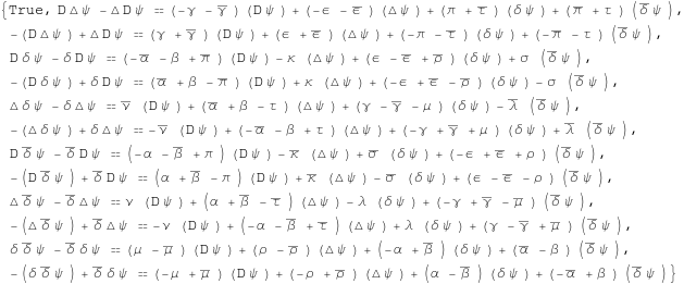
We extract the independent equations from this set.
In[172]:=
![]()
![]()
Out[172]=

These equations come in complex-conjugate pairs. Therefore we only need to consider a subset of them.
In[173]:=
![]()
In[174]:=
![]()
In[175]:=
![]()
Out[175]=

Therefore, the full set of independent commutation relations is
In[176]:=
![]()
Out[176]=

Components of the Riemann tensor in terms of the components of the curvature spinors
We are going to write the components of the Riemann tensor in the null tetrad in terms of the spinor curvature components expressed in the spin dyad. First we compute folded rules containing the independent components of each of the quantities involved.
In[177]:=
![]()
Out[177]=

In[178]:=
![]()
In[179]:=
![]()
Out[179]=

In[180]:=
![]()
In[181]:=
![]()
Out[181]=

In[182]:=
![]()
We introduce the scalars which will represent the components of the Weyl spinor
In[183]:=
![]()
![]()
![]()
![]()
![]()
![]()
![]()
![]()
![]()
![]()
![]()
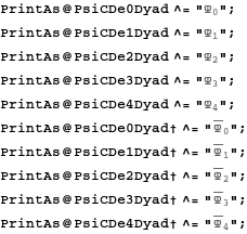
The different components of the Weyl spinor are formatted with their conventional names.
In[184]:=
In[194]:=
![]()
In[195]:=
![]()
Explicit definition of the components of the Weyl spinor.
In[196]:=

Out[196]=
![]()
In[197]:=
![]()
Out[197]=
![]()
In[198]:=
![]()
Out[198]=
![]()
In[199]:=
![]()
Out[199]=
![]()
In[200]:=
![]()
In[201]:=
![]()
We introduce the scalars which will represent the components of the Ricci spinor.
In[202]:=
![]()
![]()
![]()
![]()
![]()
![]()
![]()
![]()
![]()
![]()
![]()
![]()
![]()
![]()
![]()
![]()
![]()
![]()
![]()
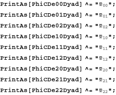
The components of the Ricci spinor are formatted with their conventional names.
In[203]:=
In[212]:=
![]()
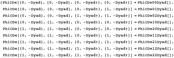
Explicit definition of the components of the Ricci spinor.
In[213]:=
Out[213]=
![]()
In[214]:=
![]()
In[215]:=
![]()
Out[215]=
![]()
In[216]:=
![]()
Out[216]=
![]()
In[217]:=
![]()
Out[217]=
![]()
In[218]:=
![]()
In[219]:=
![]()
In[220]:=
![]()
Computation of the folded rule for the Riemann tensor.
In[221]:=
![]()
In[222]:=
![]()
Next we show how to write Riemann tensor components in terms of the components of curvature spinors
In[223]:=
![]()
Out[223]=
![]()
In[224]:=
![]()
Out[224]=
![]()
In[225]:=
![]()
Out[225]=
![]()
In[226]:=
![]()
In[227]:=
![]()
In[228]:=
![]()
Out[228]=

In[229]:=
![]()
Out[229]=

We add the values just found to the folded rule containg the components of the Riemann tensor.
In[230]:=
![]()
In[231]:=
![]()
In[232]:=
![]()
From previous computations we can obtain and store the values for the components of the Ricci tensor.
In[233]:=
![]()
In[234]:=
![]()
Out[234]=
![]()
In[235]:=
![]()
Out[235]=
![]()
In[236]:=
![]()
Out[236]=
![]()
In[237]:=
![]()
Out[237]=

In[238]:=
![]()
Out[238]=

In[239]:=
![]()
In[240]:=
![]()
The scalar curvature is worked out in a similar fashion.
In[241]:=
![]()
Out[241]=
![]()
In[242]:=
![]()
Out[242]=
![]()
In[243]:=
![]()
Out[243]=
![]()
In[244]:=
![]()
Out[244]=
![]()
In[245]:=
![]()
We may also need the components of the traceless part of the Ricci tensor.
In[246]:=
![]()
In[247]:=
![]()
Out[247]=
![]()
In[248]:=
![]()
Out[248]=
![]()
In[249]:=
![]()
Out[249]=
![]()
In[250]:=
![]()
Out[250]=
![]()
In[251]:=
![]()
Out[251]=
![]()
In[252]:=
![]()
This is the complete list of the components of the Riemann tensor.
In[253]:=

Out[253]=
![]()
The Newman-Penrose equations
We now calculate the Riemann tensor with respect to the null tetrad
In[254]:=
![]()
![]()
Out[254]=
![]()
In[255]:=
![]()
Out[255]=
![]()
In[256]:=
![]()
Out[256]=
![]()
In[257]:=
![]()
Out[257]=
![]()
In[258]:=
![]()
In[259]:=
![]()
From here we obtain directly the Newman-Penrose equations
In[260]:=
![]()
In[261]:=
![]()
Out[261]=
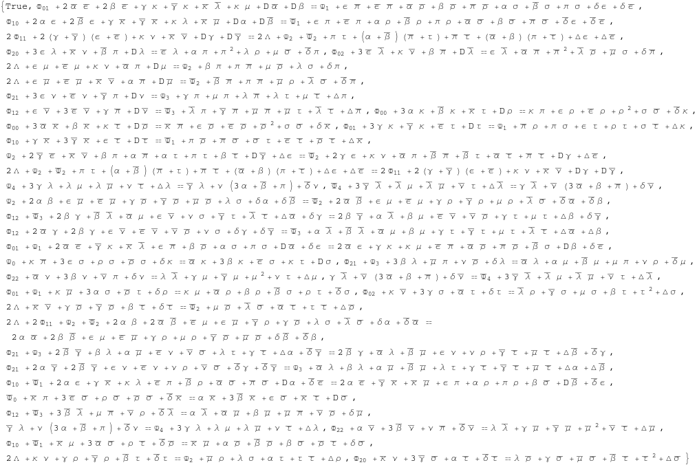
Not all the equations in this bunch are independent. To extract the independent set of equations we just eliminate a certain set of variables. The variables which we are going to eliminate are
In[262]:=
![]()
Out[262]=
![]()
In[263]:=
![]()
In[264]:=
![]()
In[265]:=
![]()
![]()
Out[265]=

In[266]:=
![]()
In[267]:=
![]()
Out[267]=

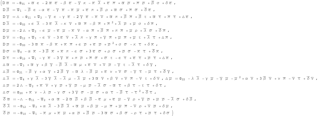
We may need the complex conjugate set in future computations.
In[268]:=
![]()
Out[268]=
In[269]:=
![]()
![]()
Out[269]=

Bianchi identities
We take next the components of the second Bianchi identity in the null tetrad.
In[270]:=
![]()
Out[270]=
![]()
In[271]:=
![]()
Out[271]=
![]()
In[272]:=
![]()
Out[272]=
![]()
In[273]:=
![]()
Out[273]=
![]()
In[274]:=
![]()
Out[274]=
![]()
In[275]:=
![]()
Out[275]=

In[276]:=
![]()
In[277]:=
![]()
In[278]:=
![]()
Not all the equations here are independent.
In[279]:=
![]()
Out[279]=
![]()
In[280]:=
![]()
Out[280]=
![]()
In[281]:=
![]()
The final result for the Bianchi identities is
In[282]:=
![]()
Out[282]=

3. The GHP formalism
The Geroch-Held-Penrose formalism (known as GHP formalism) is a particularisation of the Newman-Penrose formalism in which the spin coefficients are separated according to their boost and spin weight. Also the direcctional derivatives associated to the null tetrad are replaced by differential operators which behave well under boost and spin transformations and therefore we can speak of the boost and spin weight of these operators. This enables us to re-write the basic equations used in the Newman-Penrose formalism in terms of boost-weighted quantities only. In this section we show how this is accomplished in the framework of Spinors` and xCoba` .
Boost and spin weights
The GHP formalism only admits weighted quantities. In this subsection we introduce a command, called GHPWeightOf, which computes the boost and spin weight of any quantity. These are integers which are kept in a list. The command GHPWeightOf also checks that the GHP weight of the terms of any sum all agree, throwing an error otherwise.
In[283]:=

Weights of integers, rationals and complex numbers.
In[284]:=

Weights of products.
In[287]:=
![]()
Weights of sums
In[288]:=
![]()
Weights of powers
In[290]:=
![]()
Weights of the spin coefficients
Some of the spin coefficients are weighted quantities. These are in the following list.
In[291]:=
![]()
Out[291]=
![]()
These are the spin and boost weights of these quantities :
In[292]:=

From here we compute the weights of the complex conjugate of these quantities
In[293]:=
![]()
Out[293]=
![]()
In[294]:=
![]()
Out[294]=
![]()
Weights of the components of the curvature spinors
It is easy to deduce the weights of the components of the curvature spinors. These are their values.
In[295]:=
![]()
In[296]:=

In[297]:=

In[298]:=
![]()
GHP differential operators
The GHP differential operators are constructed by adding some extra terms to the four NP direccional derivatives. The result is a set of four differential operators having good transformation properties under spin and boost.
The GHP differential operators can be regarded as the "components" of a certain differential operator which we define next. This operator is not a true covariant derivative but just a differential operator acting on scalars, so we need to use some primitive xAct` instructions in order to create it. We use the notation ![]() as a representation for it.
as a representation for it.
In[299]:=

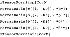
Formatting of the GHP operators with their standard symbols.
In[306]:=
The following constants represent respectively generic boost and spin weights.
In[312]:=
![]()
![]()
In[313]:=
![]()
![]()
We introduce a complex scalar of weight (p,q).
In[314]:=
![]()
![]()
![]()
We specify the weight of the scalar quantity ![]() (note that the integers w and z are zero weighted).
(note that the integers w and z are zero weighted).
In[315]:=
![]()
The action of the differential operator ![]() on a weighted scalar
on a weighted scalar ![]() is, by definition
is, by definition
In[317]:=

Out[317]=
![]()
In[318]:=
![]()
In[319]:=
![]()
In[320]:=
![]()
Out[320]=
![]()
In[321]:=
![]()
We transform previous rules in delayed rules with patterns which can be used for any weighted quantity
In[322]:=
![]()
Out[322]=
![]()
In[323]:=
![]()
Out[323]=
![]()
In[324]:=
![]()
Out[324]=

In[325]:=
![]()
Out[325]=
![]()
In[326]:=
![]()
Out[326]=
![]()
In[327]:=
![]()
Out[327]=
![]()
Each of the quantities ![]() ,
, ![]() ,
, ![]() ,
, ![]() is a spin weighted quantity. These are the specific values for the weights of each of them.
is a spin weighted quantity. These are the specific values for the weights of each of them.
In[328]:=

We also need to teach GHPWeightOf how to behave when acting on differential expressions.
In[332]:=
![]()
Commutation of the GHP differential operators
In this subsection we work out the commutation relations of each of the GHP operators. The commutator of two GHP operators is a new differential operator which acts on a generic spin weighted scalar ![]() .
.
This is the commutation between two generic GHP operators.
In[333]:=
![]()
Out[333]=
![]()
We expand this into components in order to obtain the set of commutation relations.
In[334]:=
![]()
Out[334]=

In[335]:=
![]()
Out[335]=
![]()
In[336]:=
![]()
Out[336]=
![]()
In[337]:=
![]()
Out[337]=

In[338]:=
![]()
In[339]:=
![]()
In[340]:=
![]()
Out[340]=

We use the Newman-Penrose equations on this relation.
In[341]:=
![]()
In[342]:=
![]()
In[343]:=
![]()
Out[343]=

Finally we write ![]() ,
, ![]() in terms of
in terms of ![]() ,
, ![]() and simplify the resulting expression.
and simplify the resulting expression.
In[344]:=
![]()
In[345]:=
![]()
Out[345]=

In[346]:=
![]()
We check that everything is OK
In[347]:=
![]()
Out[347]=
![]()
Ricci identities in the GHP formalism
In this subsection we use the Newman-Penrose Ricci identities (Newman-Penrose equations) to find a set of equations which only contain the GHP differential operators and spin weighted quantities. This set of equations is known as GHP equations or compacted spin coefficient equations.
These are the weighted spin coefficients.
In[348]:=
![]()
Out[348]=
![]()
These are the NP differentials of these spin coefficients.
In[349]:=
![]()
Out[349]=
![]()
We compute the GHP differentials of the weighted Newman-Penrose spin coefficients.
In[350]:=
![]()
Out[350]=

With this information we can render the Newman-Penrose equations in terms of the GHP differential operators.
In[351]:=
![]()
Out[351]=

In[352]:=
![]()
Out[352]=

We are interested in these equations which only contain weighted spin coefficients and GHP operators. These are
In[353]:=
![]()
Out[353]=

We may write these equations in an alternative way.
In[354]:=
![]()
![]()
Out[354]=

In[355]:=
![]()
Out[355]=

In[356]:=
![]()
Out[356]=

Previous set of equations is known as GHP equations or compacted spin coefficient equations.
In[357]:=
![]()
Out[357]=
![]()
Bianchi identities in the GHP formalism
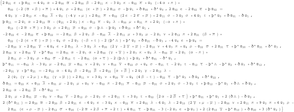
Each of the components of the curvature spinors is a weighted scalar. Using this property it is possible to rewrite the Newman-Penrose form of the Bianchi identities in terms of spin weighted quantities. This is accomplished in this subsection.
We write the differentials of the curvature components which appear in the NP Bianchi identities in terms of differentials written in ters of the GHP operators.
In[358]:=
![]()
Out[358]=
In[359]:=
![]()
Out[359]=

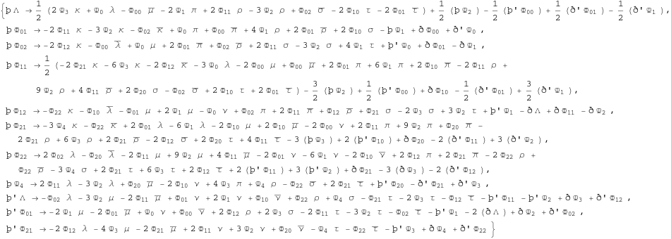
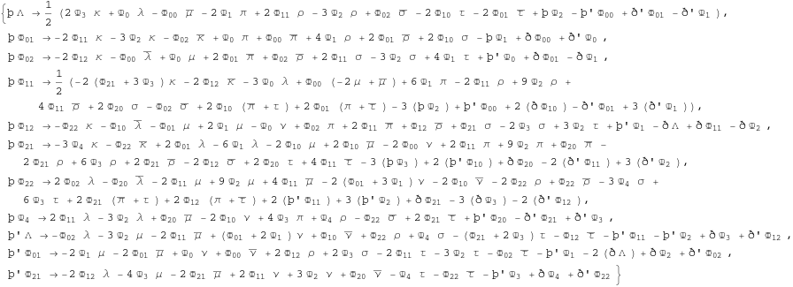
We may write these equations in an alternative way.
In[360]:=
![]()
![]()
Out[360]=
In[361]:=
![]()
Out[361]=
In[362]:=
![]()
Out[362]=

Previous set of equations is known as GHP Bianchi identities or compacted Bianchi Identities.
In[363]:=
![]()
Out[363]=
![]()
4. Quick start
In this section we show how to use in practical applications the NP and GHP equations computed in previous sections. This is intended to be a short tutorial which enables the user to start working as quick as possible with the equations of the NP and GHP formalisms, so one does not need to read the contents of previous sections to use it. However, to take full advantage of the flexibility offered by our implementation and the remaining features of xAct`, the complete knowledge of sections 1,2 and 3 is needed
The basic variables of the NP and GHP formalisms are the spin coefficients and the components of the curvature tensor. These are stored in lists.
In[364]:=
![]()
Out[364]=
![]()
In[365]:=
![]()
Out[365]=
![]()
To type any of these quantities you need to know the imput form of them. This is achieved with the Mathematica command InputForm. For example, let us display the input form of the spin coefficient ![]() :
:
In[366]:=
![]()
Out[366]//InputForm=
γDyad[]
Recall that Greek letters are typed by using the key "esc" followed by the Latin name of the letter followed by "esc". Hence
In[367]:=
![]()
Out[367]=
![]()
Other essential ingredient of the NP and GHP formalisms are the frame differentiations. In the NP formalism these are just the directional derivatives associated to the four elements of the null tetrad. To see how they are typed, we consider their action on the spin coefficient ![]() .
.
In[368]:=
![]()
Out[368]=
![]()
The head PDNP denotes a generic NP operator associated to the null tetrad, whereas the arguments {1,-NP}, ... {4,-NP} are used to refer to each of the directional derivatives of the null tetrad elements. In this way {1,-NP} means the first element of the null tetrad, {2,-NP} the second element and so on. The elements of the null tetrad are numbered according to the usual convention. In the case of the GHP formalism, we have to take into account that only weighted quantities appear in the formalism. All the components of the Riemann tensor are weighted, but not all the spin coefficients are so. The weighted spin coefficients are stored in the following list.
In[369]:=
![]()
Out[369]=
![]()
Let us take ![]() : the action of the four GHP operators on it is
: the action of the four GHP operators on it is
In[370]:=
![]()
Out[370]=
![]()
In this case, the head Θ (typed esc-Q-esc) is the notation for a generic GHP differential operator while
{1,-NP},..,{4,-NP} are, as before, the labels for each of the elements of the null tetrad. We can transform the GHP differentials into NP differentials as follows.
In[371]:=
![]()
Out[371]=
![]()
NP differentials can be also transformed back into GHP differentials.
In[372]:=
![]()
Out[372]=
![]()
In[373]:=
![]()
Out[373]=
![]()
Previous operations can be performed on any weighted quantity and the appropriate weights will be automatically inserted. For example:
In[374]:=
![]()
Out[374]=
![]()
In[375]:=
![]()
Out[375]=
![]()
The basic equations of each formalism are stored in lists. These are the names of the lists and the correspondences:
Newman-Penrose commutation relations:
In[376]:=
![]()
Out[376]=

Newman-Penrose Ricci identities:
In[377]:=
![]()
Out[377]=

Newman-Penrose Bianchi identities:
In[378]:=
![]()
Out[378]=

GHP commutators acting on a generic quantity ![]() of boost weight w and spin weight z.
of boost weight w and spin weight z.
In[379]:=
![]()
Out[379]=

GHP Ricci identities:
In[380]:=
![]()
Out[380]=

GHP Bianchi identities:
In[381]:=
![]()
Out[381]=

Within the GHP formalism any expression must be weighted. The command GHPWeightOf will compute the weight of any expression.
In[382]:=
![]()
For example: take one of the GHP Bianchi identities:
In[383]:=
![]()
Out[383]=
![]()
We compute the GHP weight of the right hand side of this relation.
In[384]:=
![]()
Out[384]=
![]()
Finally we explain how to compute the action of the GHP commutators on any quantity. For example suppose that we wish to compute the commutation of þ and ð' on the scalar ![]() . First of all, we look up in the list of GHP commutators the commutation relation we wish to use. In our case this is
. First of all, we look up in the list of GHP commutators the commutation relation we wish to use. In our case this is
In[385]:=
![]()
Out[385]=
![]()
Next we replace ![]() by
by ![]() and the weights {w, z} by their values. This is accomplished as follows
and the weights {w, z} by their values. This is accomplished as follows
In[386]:=
![]()
Out[386]=
![]()